Sensitivity Analysis in Python

This guide is organized in the following sections:

• Sensitivity Analysis Theory

• The Hard Way

• The Easy Way (use ``sensitivity`) <#Using-The-Sensitivity-Library>`__

What is Sensitivity Analysis?

Sensitivity Analysis is the process of passing different inputs to a model to see how the outputs change. It differs from Monte Carlo Simulation in that no probability distributions are assigned to the inputs, and typically larger ranges of the inputs are chosen. The purpose of Sensitivity Analysis is to understand how the outputs change over the full range of possible inputs. Sensitivity Analysis does not derive any expected outcome or a probability distribution of outcomes, instead returning a range of possible output values associated with each set of inputs.

The general process for Sensitivity Analysis is as follows:

For the model given by:

\[y = f(X)\]

\[X = [x_1, x_2, ..., x_n]\]

Where:

• \(y\): Model output

• \(X\): Model input matrix

• \(x_i\) Value if \(i\)th \(x\) variable

Follow the following steps:

• Choose a set of values for each \(x_i\)

• Take the cartesian product of these values as \([X_1, X_2, ..., X_m]\)

• For each \(X_i\), calculate \(y_i = f(X_i)\)

• Store the values of \(X_i\) mapped to \(y_i\)

• Visualize \(y_i\) versus \(X_i\)

How to Do Sensitivity Analysis in Python?

Abstract algorithms are great, but let’s see the code that can make this happen. First we’ll import pandas to use later and define a function which represents the model:

import pandas as pd

def my_model(x_1, x_2):
    """
    Represents f from above
    """
    return x_1 ** x_2

We can run this model once to get a single result:

y = my_model(2, 4)
y

16

Now let’s go step by step through the above algorithm. First let’s choose a set of values for each \(x_i\):

x1_values = [10, 20, 30]
x2_values = [1, 2, 3]

While we can use itertools.product to take a cartesian product of an arbitrary number of inputs, a more straightforward approach is to use nested for loops. A for loop within a for loop will run with each combination of the inputs.

for x1 in x1_values:
    for x2 in x2_values:
        print(x1, x2)

10 1
10 2
10 3
20 1
20 2
20 3
30 1
30 2
30 3

Now we have each \(X_i\), we need to calculate \(y_i = f(X_i)\):

for x1 in x1_values:
    for x2 in x2_values:
        y_i = my_model(x1, x2)
        print(y_i)

10
100
1000
20
400
8000
30
900
27000

Now store the values of \(X_i\) mapped to \(y_i\):

outputs = []
for x1 in x1_values:
    for x2 in x2_values:
        y_i = my_model(x1, x2)
        outputs.append((x1, x2, y_i))
outputs

[(10, 1, 10), (10, 2, 100), (10, 3, 1000), (20, 1, 20), (20, 2, 400), (20, 3, 8000), (30, 1, 30), (30, 2, 900), (30, 3, 27000)]

Now the last is to visualize the result. We can do this with a table format through a DataFrame:

df = pd.DataFrame(outputs, columns=['x_1', 'x_2', 'y'])
df

	x_1	x_2	y
0	10	1	10
1	10	2	100
2	10	3	1000
3	20	1	20
4	20	2	400
5	20	3	8000
6	30	1	30
7	30	2	900
8	30	3	27000

We can add some styling to the DataFrame to highlight the high and low values:

df.style.background_gradient(subset='y', cmap='RdYlGn')

	x_1	x_2	y
0	10	1	10
1	10	2	100
2	10	3	1000
3	20	1	20
4	20	2	400
5	20	3	8000
6	30	1	30
7	30	2	900
8	30	3	27000

We can plot the result as well with a hex-bin plot.

df.plot.hexbin(x='x_1', y='x_2', C='y', gridsize=3, cmap='RdYlGn', sharex=False)

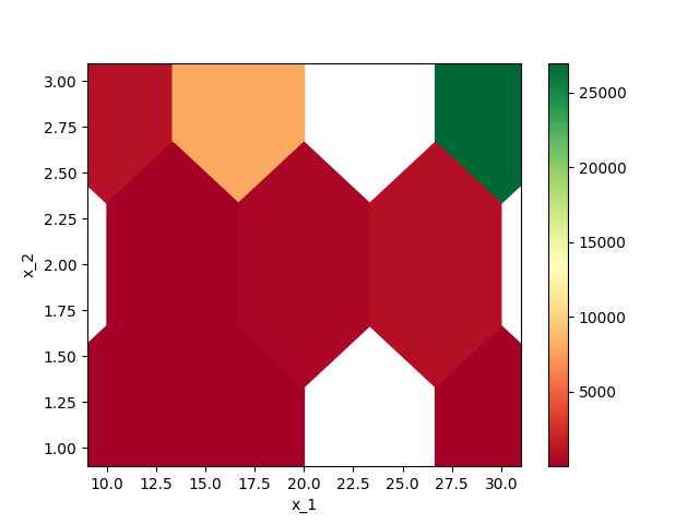
<AxesSubplot: xlabel='x_1', ylabel='x_2'>

Using The Sensitivity Library

The sensitivity package is designed around making this whole process easier. It is also able to handle more than two varying inputs with ease. The basic usage is to construct a dictionary where the keys are the names of inputs in a function and values are iterables of the values for that input. Then this dictionary is passed to SensitivityAnalyzer along with the function. The rest is handled for you.

from sensitivity import SensitivityAnalyzer

sensitivity_dict = {
    'x_1': [10, 20, 30],
    'x_2': [1, 2, 3]
}

sa = SensitivityAnalyzer(sensitivity_dict, my_model)

  0%|          | 0/9 [00:00<?, ?it/s]
100%|##########| 9/9 [00:00<00:00, 1136.50it/s]

Now that we have created the SensitivityAnalyzer object, it has finished the sensitivity analysis. We can view a DataFrame with the results at .df:

sa.df

	x_1	x_2	Result
0	10	1	10
1	10	2	100
2	10	3	1000
3	20	1	20
4	20	2	400
5	20	3	8000
6	30	1	30
7	30	2	900
8	30	3	27000

We can also get the hex-bin plot and styled DataFrame:

plot = sa.plot()

styled = sa.styled_dfs()

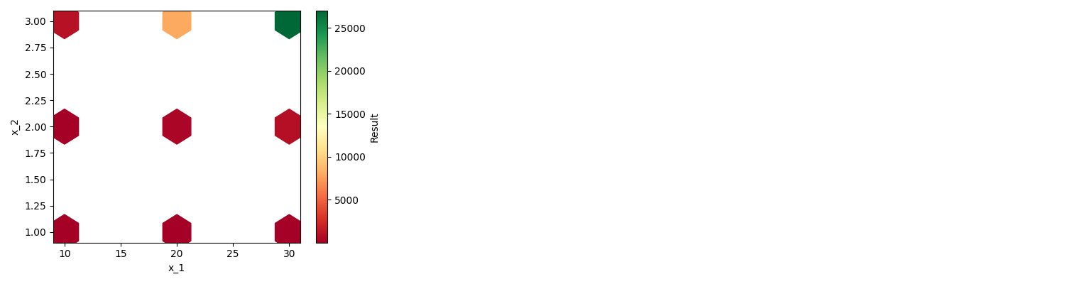
<IPython.core.display.HTML object>
<IPython.core.display.HTML object>

When creating the SensitivityAnalyzer object, you can pass other options for formatting the outputs:

labels = {
    'x_1': 'First Input',
    'x_2': 'Second Input'
}

sa = SensitivityAnalyzer(
    sensitivity_dict, my_model, grid_size=3, reverse_colors=True, color_map='coolwarm', labels=labels
)
plot = sa.plot()

styled = sa.styled_dfs()

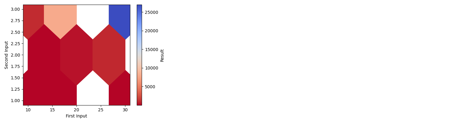
  0%|          | 0/9 [00:00<?, ?it/s]
100%|##########| 9/9 [00:00<00:00, 1167.35it/s]
<IPython.core.display.HTML object>
<IPython.core.display.HTML object>

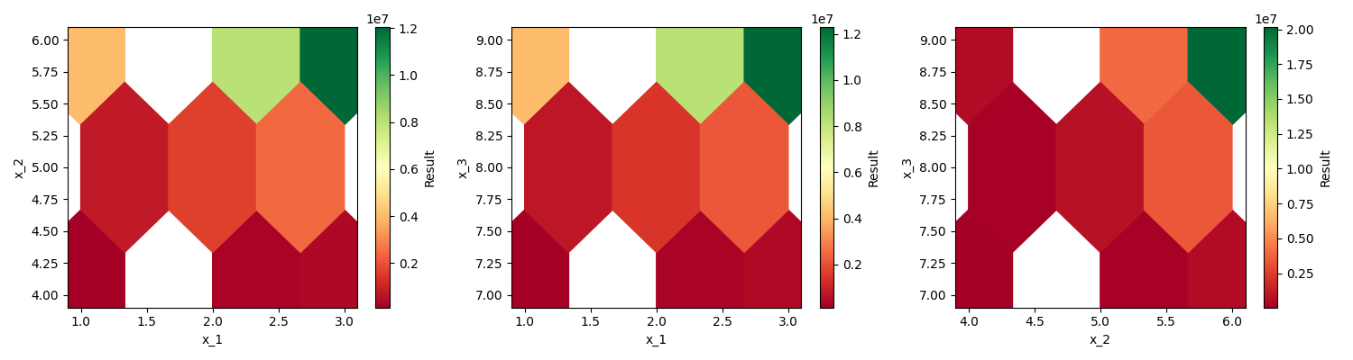
This all works with more than two inputs as well. In that case we will get multiple pair-wise plots and styled DataFrames:

def my_model_2(x_1, x_2, x_3):
    return x_1 * x_2 ** x_3

sensitivity_dict = {
    'x_1': [1, 2, 3],
    'x_2': [4, 5, 6],
    'x_3': [7, 8, 9]
}

sa = SensitivityAnalyzer(sensitivity_dict, my_model_2, grid_size=3)

plot = sa.plot()

styled_dict = sa.styled_dfs()

  0%|          | 0/27 [00:00<?, ?it/s]
100%|##########| 27/27 [00:00<00:00, 1181.84it/s]
<IPython.core.display.HTML object>
<IPython.core.display.HTML object>
<IPython.core.display.HTML object>
<IPython.core.display.HTML object>
<IPython.core.display.HTML object>
<IPython.core.display.HTML object>

The plot is still a single Figure object, but the styled_dfs produces a dictionary where there are more than two inputs. The keys of the dictionary are a tuple of the column names involved in the Styler, and the values are the Stylers.

styled_dict

{('x_1', 'x_2'): <pandas.io.formats.style.Styler object at 0x7f8dac269fd0>, ('x_1', 'x_3'): <pandas.io.formats.style.Styler object at 0x7f8dac203be0>, ('x_2', 'x_3'): <pandas.io.formats.style.Styler object at 0x7f8dac2e32b0>}

Adding Additional Styling to Styled DataFrames

It could be desired to pass some number or other formatting to the styled DataFrames. This can be done with the num_fmt argument, either when first creating the SensitivityAnalyzer or when calling the styled_dfs method. Just pass it the string of the number format, in the same way you would specify the number formatting string for df.style.format.

styled_dict = sa.styled_dfs(num_fmt='${:,.0f}')

<IPython.core.display.HTML object>
<IPython.core.display.HTML object>
<IPython.core.display.HTML object>
<IPython.core.display.HTML object>
<IPython.core.display.HTML object>
<IPython.core.display.HTML object>