Note

Click here to download the full example code or to run this example in your browser via Binder

Data Management in Python Using Standard Tooling¶

Prior to beginning the tutorial, please install the following packages via pip:

pandas
matplotlib
statsmodels
seaborn
openpyxl
xlrd

Note: if you’re using Anaconda, some of these will be installed already.

Note: if you’re running the example in Binder, no installation is necessary

Overview¶

pandas is a large library which includes a data structure called a DataFrame which is originally based on R’s data.frame. In Python, it is built on top of the array datatype in the similarly popular numpy library. Each column in a DataFrame is a pandas Series.

I use numpy for some specific functions or when I need higher performance than pandas, but pandas is much more convenient to use.

Here is what we’re going to cover:

**Selecting Data**
**Aggregating**
**Merging**
**Time series**
**Plotting**
**Regressions**
**Input and Output**

Give me a `DataFrame`!¶

A DataFrame can be created in many ways, including: - From a csv or Excel file - From a SAS7BDAT (SAS data) or dta (Stata data) file - From other Python data structures (list of tuples, dictionaries, numpy arrays)

Here I will create an example DataFrame from a list of tuples. At the end I will show loading and writing to files.

import pandas as pd #this is the convention for importing pandas, then you can use pd. for functions

df = pd.DataFrame(
    data=[
        ('Walmart', 'FL', '1/2/2000', .02),
        ('Walmart', 'FL', '1/3/2000', .03),
        ('Walmart', 'FL', '1/4/2000', .04),
        ('Trader Joes', 'GA', '1/2/2000', .06),
        ('Trader Joes', 'GA', '1/3/2000', .07),
        ('Trader Joes', 'GA', '1/4/2000', .08),
        ('Publix', 'FL', '1/2/2000', .1),
        ('Publix', 'FL', '1/3/2000', .11),
        ('Publix', 'FL', '1/4/2000', .12),
    ],
    columns = ['Company', 'State', 'Date', 'Return']
)

pandas combined with Jupyter gives you a nice representation of your data by simply typing the name of the variable storing your DataFrame:

df

	Company	State	Date	Return
0	Walmart	FL	1/2/2000	0.02
1	Walmart	FL	1/3/2000	0.03
2	Walmart	FL	1/4/2000	0.04
3	Trader Joes	GA	1/2/2000	0.06
4	Trader Joes	GA	1/3/2000	0.07
5	Trader Joes	GA	1/4/2000	0.08
6	Publix	FL	1/2/2000	0.10
7	Publix	FL	1/3/2000	0.11
8	Publix	FL	1/4/2000	0.12

Working with Data in Pandas¶

One of the DataFrames greatest strengths is how flexibly they can be split, combined, and aggregated.

Selecting Data¶

df[df['State'] == 'FL'] # read: dataframe where the dataframe column 'state' is 'FL'

df.iloc[1:3] # give me the second through the third rows

df.iloc[:, 2] # all rows for the third column (looks different because it's a Series)

df['Company'] # company column (Series)

best_grocery_stores = ['Trader Joes', 'Publix']
# only rows where company is in the best grocery stores and has a high return,
# but also give me only the company and return columns
df.loc[df['Company'].isin(best_grocery_stores) & (df['Return'] > 0.07), ['Company', 'Return']]

	Company	Return
5	Trader Joes	0.08
6	Publix	0.10
7	Publix	0.11
8	Publix	0.12

Aggregating¶

DataFrames have a .groupby which works similarly to group by in a SQL (proc SQL) command.

df.groupby('Company')

Out:

<pandas.core.groupby.generic.DataFrameGroupBy object at 0x7f27a2dd8fd0>

To make it useful, we must aggregate the data somehow:

df.groupby(['State','Date']).mean() #also .median, .std, .count

		Return
State	Date
FL	1/2/2000	0.06
	1/3/2000	0.07
	1/4/2000	0.08
GA	1/2/2000	0.06
	1/3/2000	0.07
	1/4/2000	0.08

Note that there the index becomes the groupby columns. If we want keep the columns in the DataFrame, pass as_index=False.

df.groupby(['State','Date'], as_index=False).mean() #also .median, .std, .count

	State	Date	Return
0	FL	1/2/2000	0.06
1	FL	1/3/2000	0.07
2	FL	1/4/2000	0.08
3	GA	1/2/2000	0.06
4	GA	1/3/2000	0.07
5	GA	1/4/2000	0.08

Note that the shape of the data when using plain groupby is whatever the shape of the unique values of the groupby columns. If instead we want to add a column to our DataFrame representing the aggregated values, use .transform on top of groupby.

This example also shows how to assign a new column to a DataFrame.

df['State Return Average'] = df.groupby(['State','Date']).transform('mean')
df

	Company	State	Date	Return	State Return Average
0	Walmart	FL	1/2/2000	0.02	0.06
1	Walmart	FL	1/3/2000	0.03	0.07
2	Walmart	FL	1/4/2000	0.04	0.08
3	Trader Joes	GA	1/2/2000	0.06	0.06
4	Trader Joes	GA	1/3/2000	0.07	0.07
5	Trader Joes	GA	1/4/2000	0.08	0.08
6	Publix	FL	1/2/2000	0.10	0.06
7	Publix	FL	1/3/2000	0.11	0.07
8	Publix	FL	1/4/2000	0.12	0.08

Columns can be combined with basic math operations

df['Ratio'] = df['Return'] / df['State Return Average']
df

	Company	State	Date	Return	State Return Average	Ratio
0	Walmart	FL	1/2/2000	0.02	0.06	0.333333
1	Walmart	FL	1/3/2000	0.03	0.07	0.428571
2	Walmart	FL	1/4/2000	0.04	0.08	0.500000
3	Trader Joes	GA	1/2/2000	0.06	0.06	1.000000
4	Trader Joes	GA	1/3/2000	0.07	0.07	1.000000
5	Trader Joes	GA	1/4/2000	0.08	0.08	1.000000
6	Publix	FL	1/2/2000	0.10	0.06	1.666667
7	Publix	FL	1/3/2000	0.11	0.07	1.571429
8	Publix	FL	1/4/2000	0.12	0.08	1.500000

Functions can be applied to columns or the entire DataFrame:

import numpy as np # convention for importing numpy.

def sort_ratios(value):

    # If the value is missing or is not a number, return as is
    # Without this, the function will error out as soon as it hits either of those
    if pd.isnull(value) or not isinstance(value, np.float):
        return value

    # Otherwise, sort into categories based on the value
    if value == 1:
        return 'Even'
    if value < 1:
        return 'Low'
    if value >= 1:
        return 'High'

df['Ratio Size'] = df['Ratio'].apply(sort_ratios) # apply function to ratio column, save result as ratio size column
df

df.applymap(sort_ratios) # apply function to all values in df, but only display and don't save back to df

	Company	State	Date	Return	State Return Average	Ratio	Ratio Size
0	Walmart	FL	1/2/2000	Low	Low	Low	Low
1	Walmart	FL	1/3/2000	Low	Low	Low	Low
2	Walmart	FL	1/4/2000	Low	Low	Low	Low
3	Trader Joes	GA	1/2/2000	Low	Low	Even	Even
4	Trader Joes	GA	1/3/2000	Low	Low	Even	Even
5	Trader Joes	GA	1/4/2000	Low	Low	Even	Even
6	Publix	FL	1/2/2000	Low	Low	High	High
7	Publix	FL	1/3/2000	Low	Low	High	High
8	Publix	FL	1/4/2000	Low	Low	High	High

Merging¶

See here for more details.

Let’s create a DataFrame containing information on employment rates in the various states and merge it to this dataset.

employment_df = pd.DataFrame(
    data=[
        ('FL', 0.06),
        ('GA', 0.08),
        ('PA', 0.07)
    ],
    columns=['State', 'Unemployment']
)
employment_df

df = df.merge(employment_df, how='left', on='State')
df

	Company	State	Date	Return	State Return Average	Ratio	Ratio Size	Unemployment
0	Walmart	FL	1/2/2000	0.02	0.06	0.333333	Low	0.06
1	Walmart	FL	1/3/2000	0.03	0.07	0.428571	Low	0.06
2	Walmart	FL	1/4/2000	0.04	0.08	0.500000	Low	0.06
3	Trader Joes	GA	1/2/2000	0.06	0.06	1.000000	Even	0.08
4	Trader Joes	GA	1/3/2000	0.07	0.07	1.000000	Even	0.08
5	Trader Joes	GA	1/4/2000	0.08	0.08	1.000000	Even	0.08
6	Publix	FL	1/2/2000	0.10	0.06	1.666667	High	0.06
7	Publix	FL	1/3/2000	0.11	0.07	1.571429	High	0.06
8	Publix	FL	1/4/2000	0.12	0.08	1.500000	High	0.06

Appending is similarly simple. Here I will append a slightly modified DataFrame to itself:

copy_df = df.copy()
copy_df['Extra Column'] = 5
copy_df.drop('Ratio Size', axis=1, inplace=True) # inplace=True means it gets dropped in the existing DataFrame
df.append(copy_df)

	Company	State	Date	Return	State Return Average	Ratio	Ratio Size	Unemployment	Extra Column
0	Walmart	FL	1/2/2000	0.02	0.06	0.333333	Low	0.06	NaN
1	Walmart	FL	1/3/2000	0.03	0.07	0.428571	Low	0.06	NaN
2	Walmart	FL	1/4/2000	0.04	0.08	0.500000	Low	0.06	NaN
3	Trader Joes	GA	1/2/2000	0.06	0.06	1.000000	Even	0.08	NaN
4	Trader Joes	GA	1/3/2000	0.07	0.07	1.000000	Even	0.08	NaN
5	Trader Joes	GA	1/4/2000	0.08	0.08	1.000000	Even	0.08	NaN
6	Publix	FL	1/2/2000	0.10	0.06	1.666667	High	0.06	NaN
7	Publix	FL	1/3/2000	0.11	0.07	1.571429	High	0.06	NaN
8	Publix	FL	1/4/2000	0.12	0.08	1.500000	High	0.06	NaN
0	Walmart	FL	1/2/2000	0.02	0.06	0.333333	NaN	0.06	5.0
1	Walmart	FL	1/3/2000	0.03	0.07	0.428571	NaN	0.06	5.0
2	Walmart	FL	1/4/2000	0.04	0.08	0.500000	NaN	0.06	5.0
3	Trader Joes	GA	1/2/2000	0.06	0.06	1.000000	NaN	0.08	5.0
4	Trader Joes	GA	1/3/2000	0.07	0.07	1.000000	NaN	0.08	5.0
5	Trader Joes	GA	1/4/2000	0.08	0.08	1.000000	NaN	0.08	5.0
6	Publix	FL	1/2/2000	0.10	0.06	1.666667	NaN	0.06	5.0
7	Publix	FL	1/3/2000	0.11	0.07	1.571429	NaN	0.06	5.0
8	Publix	FL	1/4/2000	0.12	0.08	1.500000	NaN	0.06	5.0

We can append to the side as well! (concatenate)

temp_df = pd.concat([df, copy_df], axis=1)
temp_df

	Company	State	Date	Return	State Return Average	Ratio	Ratio Size	Unemployment	Company	State	Date	Return	State Return Average	Ratio	Unemployment	Extra Column
0	Walmart	FL	1/2/2000	0.02	0.06	0.333333	Low	0.06	Walmart	FL	1/2/2000	0.02	0.06	0.333333	0.06	5
1	Walmart	FL	1/3/2000	0.03	0.07	0.428571	Low	0.06	Walmart	FL	1/3/2000	0.03	0.07	0.428571	0.06	5
2	Walmart	FL	1/4/2000	0.04	0.08	0.500000	Low	0.06	Walmart	FL	1/4/2000	0.04	0.08	0.500000	0.06	5
3	Trader Joes	GA	1/2/2000	0.06	0.06	1.000000	Even	0.08	Trader Joes	GA	1/2/2000	0.06	0.06	1.000000	0.08	5
4	Trader Joes	GA	1/3/2000	0.07	0.07	1.000000	Even	0.08	Trader Joes	GA	1/3/2000	0.07	0.07	1.000000	0.08	5
5	Trader Joes	GA	1/4/2000	0.08	0.08	1.000000	Even	0.08	Trader Joes	GA	1/4/2000	0.08	0.08	1.000000	0.08	5
6	Publix	FL	1/2/2000	0.10	0.06	1.666667	High	0.06	Publix	FL	1/2/2000	0.10	0.06	1.666667	0.06	5
7	Publix	FL	1/3/2000	0.11	0.07	1.571429	High	0.06	Publix	FL	1/3/2000	0.11	0.07	1.571429	0.06	5
8	Publix	FL	1/4/2000	0.12	0.08	1.500000	High	0.06	Publix	FL	1/4/2000	0.12	0.08	1.500000	0.06	5

Be careful, pandas allows you to have multiple columns with the same name (generally a bad idea):

temp_df['Unemployment']

	Unemployment	Unemployment
0	0.06	0.06
1	0.06	0.06
2	0.06	0.06
3	0.08	0.08
4	0.08	0.08
5	0.08	0.08
6	0.06	0.06
7	0.06	0.06
8	0.06	0.06

Time series¶

See here for more details.

Lagging¶

Lags are easy with pandas. The number in shift below represents the number of rows to lag.

df.sort_values(['Company', 'Date'], inplace=True)
df['Lag Return'] = df['Return'].shift(1)
df

	Company	State	Date	Return	State Return Average	Ratio	Ratio Size	Unemployment	Lag Return
6	Publix	FL	1/2/2000	0.10	0.06	1.666667	High	0.06	NaN
7	Publix	FL	1/3/2000	0.11	0.07	1.571429	High	0.06	0.10
8	Publix	FL	1/4/2000	0.12	0.08	1.500000	High	0.06	0.11
3	Trader Joes	GA	1/2/2000	0.06	0.06	1.000000	Even	0.08	0.12
4	Trader Joes	GA	1/3/2000	0.07	0.07	1.000000	Even	0.08	0.06
5	Trader Joes	GA	1/4/2000	0.08	0.08	1.000000	Even	0.08	0.07
0	Walmart	FL	1/2/2000	0.02	0.06	0.333333	Low	0.06	0.08
1	Walmart	FL	1/3/2000	0.03	0.07	0.428571	Low	0.06	0.02
2	Walmart	FL	1/4/2000	0.04	0.08	0.500000	Low	0.06	0.03

But really we want the lagged value to come from the same firm:

df['Lag Return'] = df.groupby('Company')['Return'].shift(1)
df

	Company	State	Date	Return	State Return Average	Ratio	Ratio Size	Unemployment	Lag Return
6	Publix	FL	1/2/2000	0.10	0.06	1.666667	High	0.06	NaN
7	Publix	FL	1/3/2000	0.11	0.07	1.571429	High	0.06	0.10
8	Publix	FL	1/4/2000	0.12	0.08	1.500000	High	0.06	0.11
3	Trader Joes	GA	1/2/2000	0.06	0.06	1.000000	Even	0.08	NaN
4	Trader Joes	GA	1/3/2000	0.07	0.07	1.000000	Even	0.08	0.06
5	Trader Joes	GA	1/4/2000	0.08	0.08	1.000000	Even	0.08	0.07
0	Walmart	FL	1/2/2000	0.02	0.06	0.333333	Low	0.06	NaN
1	Walmart	FL	1/3/2000	0.03	0.07	0.428571	Low	0.06	0.02
2	Walmart	FL	1/4/2000	0.04	0.08	0.500000	Low	0.06	0.03

Things get slightly more complicated if you want to take into account missing dates within a firm. Then you must fill the DataFrame with missing data for those excluded dates, then run the above function, then drop those missing rows. A bit too much for this tutorial, but I have code available for this upon request.

Resampling¶

pandas has a lot of convenient methods for changing the frequency of the data.

Here I will create a df containing intraday returns for the three companies

import datetime
from itertools import product

firms = df['Company'].unique().tolist() # list of companies in df
dates = df['Date'].unique().tolist() # list of dates in df
num_periods_per_day = 13 #30 minute intervals
combos = product(firms, dates, [i+1 for i in range(num_periods_per_day)]) # all combinations of company, date, and period number
data_tuples = [
    (
        combo[0], # company
        datetime.datetime.strptime(combo[1], '%m/%d/%Y') + datetime.timedelta(hours=9.5, minutes=30 * combo[2]), #datetime
        np.random.rand() * 100 # price
    )
    for combo in combos
]
intraday_df = pd.DataFrame(data_tuples, columns=['Company', 'Datetime', 'Price'])
intraday_df.head() # now the df is quite long, so we can use df.head() and df.tail() to see beginning and end of df

	Company	Datetime	Price
0	Publix	2000-01-02 10:00:00	25.250127
1	Publix	2000-01-02 10:30:00	78.297648
2	Publix	2000-01-02 11:00:00	18.903450
3	Publix	2000-01-02 11:30:00	42.139811
4	Publix	2000-01-02 12:00:00	53.523835

First must set the date variable as the index to do resampling

intraday_df.set_index('Datetime', inplace=True)

Now we can resample to aggregate:

intraday_df.groupby('Company').resample('1D').mean()

		Price
Company	Datetime
Publix	2000-01-02	51.581870
	2000-01-03	49.985571
	2000-01-04	49.441363
Trader Joes	2000-01-02	44.736422
	2000-01-03	59.731791
	2000-01-04	38.360582
Walmart	2000-01-02	65.725321
	2000-01-03	50.844221
	2000-01-04	42.806827

Or we can increase the frequency of the data, using bfill to backward fill or ffill to forward fill. Here I specify to backward fill but only go back one period at most.

intraday_df.groupby('Company').resample('10min').bfill(limit=1).head(10)

		Company	Price
Company	Datetime
Publix	2000-01-02 10:00:00	Publix	25.250127
	2000-01-02 10:10:00	NaN	NaN
	2000-01-02 10:20:00	Publix	78.297648
	2000-01-02 10:30:00	Publix	78.297648
	2000-01-02 10:40:00	NaN	NaN
	2000-01-02 10:50:00	Publix	18.903450
	2000-01-02 11:00:00	Publix	18.903450
	2000-01-02 11:10:00	NaN	NaN
	2000-01-02 11:20:00	Publix	42.139811
	2000-01-02 11:30:00	Publix	42.139811

Plotting¶

Oh yeah, we’ve got graphs too. pandas’ plotting functionality is built on top of the popular matplotlib library, which is a graphing library based on MATLAB’s graphing functionality.

# we've got to run this magic once per session if we want graphics to show up in the notebook
# %matplotlib inline

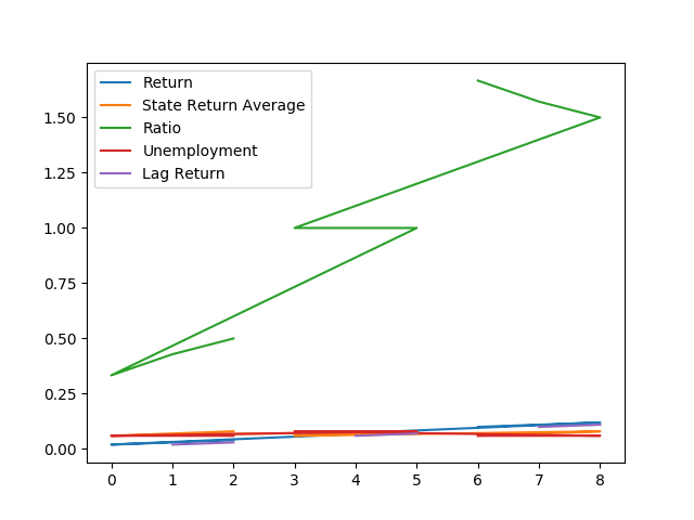
pandas tries to guess what you want to plot. By default it will put each numeric column as a y variable and the index as the x variable.

df.plot()

../_images/sphx_glr_data_management_in_python_001.png

Out:

<matplotlib.axes._subplots.AxesSubplot object at 0x7f27a2a72690>

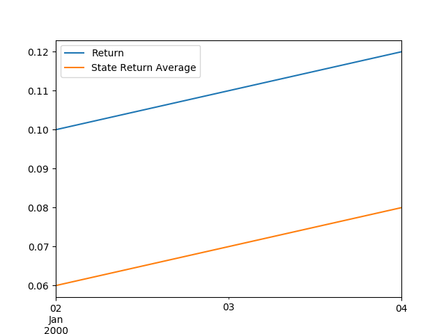
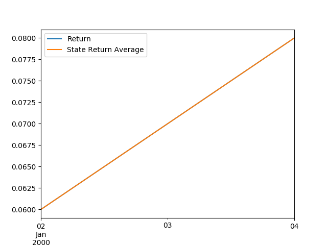
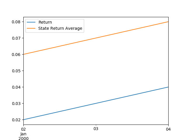
But we can tell it specifically what we want to do. Maybe we want one plot for each company showing only how the company return moves relative to the state average return over time.

df

df['Date'] = pd.to_datetime(df['Date']) # convert date from string type to datetime type
df.groupby('Company').plot(y=['Return', 'State Return Average'], x='Date')

Out:

Company
Publix         AxesSubplot(0.125,0.11;0.775x0.77)
Trader Joes    AxesSubplot(0.125,0.11;0.775x0.77)
Walmart        AxesSubplot(0.125,0.11;0.775x0.77)
dtype: object

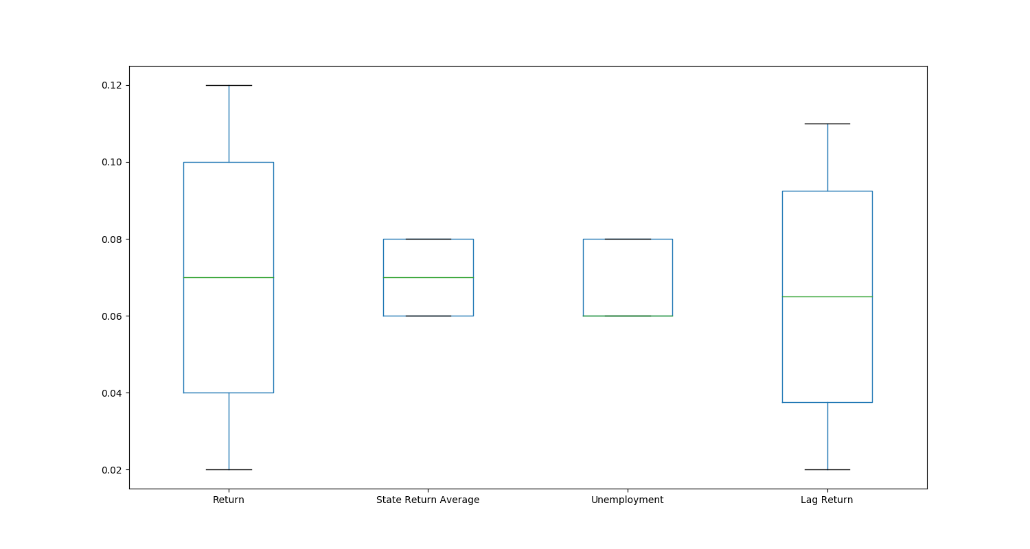
pandas exposes most of the plots in matplotlib. Supported types include: - ‘line’ : line plot (default) - ‘bar’ : vertical bar plot - ‘barh’ : horizontal bar plot - ‘hist’ : histogram - ‘box’ : boxplot - ‘kde’ : Kernel Density Estimation plot - ‘density’ : same as ‘kde’ - ‘area’ : area plot - ‘pie’ : pie plot - ‘scatter’ : scatter plot - ‘hexbin’ : hexbin plot

df.drop('Ratio', axis=1).plot(kind='box', figsize=(15,8))

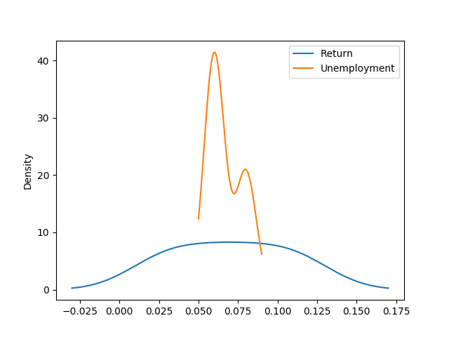
df.plot(y=['Return', 'Unemployment'], kind='kde')

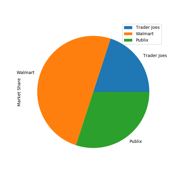
market_share_df = pd.DataFrame(
    data=[
        ('Trader Joes', .2),
        ('Walmart', .5),
        ('Publix', .3)
    ],
    columns=['Company', 'Market Share']
).set_index('Company')
market_share_df.plot(y='Market Share', kind='pie', figsize=(6,6))

Out:

<matplotlib.axes._subplots.AxesSubplot object at 0x7f2798ad9a50>

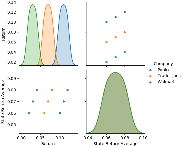
Check out the seaborn package for some cool high level plotting capabilities.

import seaborn as sns # convention for importing seaborn
sns.pairplot(df[['Company', 'Return', 'State Return Average']], hue='Company')

../_images/sphx_glr_data_management_in_python_008.png

Out:

<seaborn.axisgrid.PairGrid object at 0x7f27977cf690>

Regressions¶

Alright, we’ve got some cleaned up data. Now we can run regressions on them with the statsmodels module. Here I will show the “formula” approach to statsmodels, which is just one of the two main interfaces. The formula approach will feel similar to specifying a regression in R or Stata. However we can also directly pass DataFrames containing the y and x variables rather than specifying a formula.

df

import statsmodels.formula.api as smf # convention for importing statsmodels

model = smf.ols(formula="Return ~ Unemployment", data=df)
result = model.fit()
result.summary()

Out:

/home/runner/.local/share/virtualenvs/py-research-workflows-rjN0B_bW/lib/python3.7/site-packages/scipy/stats/stats.py:1535: UserWarning: kurtosistest only valid for n>=20 ... continuing anyway, n=9
  "anyway, n=%i" % int(n))

OLS Regression Results
Dep. Variable:	Return	R-squared:	0.000
Model:	OLS	Adj. R-squared:	-0.143
Method:	Least Squares	F-statistic:	0.000
Date:	Wed, 19 Feb 2020	Prob (F-statistic):	1.00
Time:	15:02:22	Log-Likelihood:	17.751
No. Observations:	9	AIC:	-31.50
Df Residuals:	7	BIC:	-31.11
Df Model:	1
Covariance Type:	nonrobust

	coef	std err	t	P>\|t\|	[0.025	0.975]
Intercept	0.0700	0.091	0.770	0.466	-0.145	0.285
Unemployment	5.551e-16	1.350	4.11e-16	1.000	-3.191	3.191

Omnibus:	1.292	Durbin-Watson:	0.765
Prob(Omnibus):	0.524	Jarque-Bera (JB):	0.667
Skew:	0.000	Prob(JB):	0.716
Kurtosis:	1.666	Cond. No.	107.

Warnings:
[1] Standard Errors assume that the covariance matrix of the errors is correctly specified.

Looks like a regression summary should. We can also use fixed effects and interaction terms. Here showing fixed effects:

df.rename(columns={'Ratio Size': 'ratio_size'}, inplace=True) # statsmodels formula doesn't like spaces in column names
model2 = smf.ols(formula="Return ~ Unemployment + C(ratio_size)", data=df)
result2 = model2.fit()
result2.summary()

OLS Regression Results
Dep. Variable:	Return	R-squared:	0.941
Model:	OLS	Adj. R-squared:	0.922
Method:	Least Squares	F-statistic:	48.00
Date:	Wed, 19 Feb 2020	Prob (F-statistic):	0.000204
Time:	15:02:22	Log-Likelihood:	30.501
No. Observations:	9	AIC:	-55.00
Df Residuals:	6	BIC:	-54.41
Df Model:	2
Covariance Type:	nonrobust

	coef	std err	t	P>\|t\|	[0.025	0.975]
Intercept	0.0696	0.006	12.163	0.000	0.056	0.084
C(ratio_size)[T.High]	0.0401	0.008	4.919	0.003	0.020	0.060
C(ratio_size)[T.Low]	-0.0399	0.008	-4.892	0.003	-0.060	-0.020
Unemployment	0.0056	0.001	7.867	0.000	0.004	0.007

Omnibus:	2.380	Durbin-Watson:	2.333
Prob(Omnibus):	0.304	Jarque-Bera (JB):	0.844
Skew:	-0.000	Prob(JB):	0.656
Kurtosis:	1.500	Cond. No.	3.54e+17

Warnings:
[1] Standard Errors assume that the covariance matrix of the errors is correctly specified.
[2] The smallest eigenvalue is 8.96e-35. This might indicate that there are
strong multicollinearity problems or that the design matrix is singular.

Now interaction terms

# use * for interaction keeping individual variables, : for only interaction
model3 = smf.ols(formula="Return ~ Unemployment*Ratio", data=df)
result3 = model3.fit()
result3.summary()

OLS Regression Results
Dep. Variable:	Return	R-squared:	0.928
Model:	OLS	Adj. R-squared:	0.904
Method:	Least Squares	F-statistic:	38.83
Date:	Wed, 19 Feb 2020	Prob (F-statistic):	0.000369
Time:	15:02:22	Log-Likelihood:	29.609
No. Observations:	9	AIC:	-53.22
Df Residuals:	6	BIC:	-52.63
Df Model:	2
Covariance Type:	nonrobust

	coef	std err	t	P>\|t\|	[0.025	0.975]
Intercept	0.0020	0.017	0.121	0.907	-0.039	0.043
Unemployment	-0.0020	0.195	-0.010	0.992	-0.479	0.475
Ratio	0.0680	0.014	4.849	0.003	0.034	0.102
Unemployment:Ratio	0.0020	0.195	0.010	0.992	-0.476	0.480

Omnibus:	0.037	Durbin-Watson:	2.212
Prob(Omnibus):	0.982	Jarque-Bera (JB):	0.148
Skew:	0.057	Prob(JB):	0.929
Kurtosis:	2.383	Cond. No.	1.77e+17

Warnings:
[1] Standard Errors assume that the covariance matrix of the errors is correctly specified.
[2] The smallest eigenvalue is 6.15e-34. This might indicate that there are
strong multicollinearity problems or that the design matrix is singular.

Want to throw together these models into one summary table?

from statsmodels.iolib.summary2 import summary_col

reg_list = [result, result2, result3]
summ = summary_col(
    reg_list,
    stars=True,
    info_dict = {
        'N': lambda x: "{0:d}".format(int(x.nobs)),
        'Adj-R2': lambda x: "{:.2f}".format(x.rsquared_adj)
    }
)
summ

	Return I	Return II	Return III
C(ratio_size)[T.High]		0.0401***
		(0.0082)
C(ratio_size)[T.Low]		-0.0399***
		(0.0082)
Intercept	0.0700	0.0696***	0.0020
	(0.0909)	(0.0057)	(0.0167)
R-squared	-0.1429	0.9216	0.9044
	0.0000	0.9412	0.9283
Ratio			0.0680***
			(0.0140)
Unemployment	0.0000	0.0056***	-0.0020
	(1.3496)	(0.0007)	(0.1951)
Unemployment:Ratio			0.0020
			(0.1953)
N	9	9	9
Adj-R2	-0.14	0.92	0.90

On the backend, statsmodels’ summary_col uses a DataFrame which we can access as:

summ.tables[0]

	Return I	Return II	Return III
C(ratio_size)[T.High]		0.0401***
		(0.0082)
C(ratio_size)[T.Low]		-0.0399***
		(0.0082)
Intercept	0.0700	0.0696***	0.0020
	(0.0909)	(0.0057)	(0.0167)
R-squared	-0.1429	0.9216	0.9044
	0.0000	0.9412	0.9283
Ratio			0.0680***
			(0.0140)
Unemployment	0.0000	0.0056***	-0.0020
	(1.3496)	(0.0007)	(0.1951)
Unemployment:Ratio			0.0020
			(0.1953)
N	9	9	9
Adj-R2	-0.14	0.92	0.90

Therefore we can write functions to do any cleanup we want on the summary, leveraging pandas:

def replace_fixed_effects_cols(df):
    """
    hackish way to do this just for example
    """
    out_df = df.iloc[4:] #remove fixed effect dummy rows
    out_df.loc['Ratio Size Fixed Effects'] = ('No', 'Yes', 'No')
    return out_df

clean_summ = replace_fixed_effects_cols(summ.tables[0])
clean_summ

Out:

/home/runner/.local/share/virtualenvs/py-research-workflows-rjN0B_bW/lib/python3.7/site-packages/pandas/core/indexing.py:670: SettingWithCopyWarning:
A value is trying to be set on a copy of a slice from a DataFrame

See the caveats in the documentation: https://pandas.pydata.org/pandas-docs/stable/user_guide/indexing.html#returning-a-view-versus-a-copy
  self._setitem_with_indexer(indexer, value)

	Return I	Return II	Return III
Intercept	0.0700	0.0696***	0.0020
	(0.0909)	(0.0057)	(0.0167)
R-squared	-0.1429	0.9216	0.9044
	0.0000	0.9412	0.9283
Ratio			0.0680***
			(0.0140)
Unemployment	0.0000	0.0056***	-0.0020
	(1.3496)	(0.0007)	(0.1951)
Unemployment:Ratio			0.0020
			(0.1953)
N	9	9	9
Adj-R2	-0.14	0.92	0.90
Ratio Size Fixed Effects	No	Yes	No

Pretty cool, right? Since it’s a DataFrame, we can even output it to LaTeX:

clean_summ.to_latex()

Out:

'\\begin{tabular}{llll}\n\\toprule\n{} &  Return I &  Return II & Return III \\\\\n\\midrule\nIntercept                &    0.0700 &  0.0696*** &     0.0020 \\\\\n                         &  (0.0909) &   (0.0057) &   (0.0167) \\\\\nR-squared                &   -0.1429 &     0.9216 &     0.9044 \\\\\n                         &    0.0000 &     0.9412 &     0.9283 \\\\\nRatio                    &           &            &  0.0680*** \\\\\n                         &           &            &   (0.0140) \\\\\nUnemployment             &    0.0000 &  0.0056*** &    -0.0020 \\\\\n                         &  (1.3496) &   (0.0007) &   (0.1951) \\\\\nUnemployment:Ratio       &           &            &     0.0020 \\\\\n                         &           &            &   (0.1953) \\\\\nN                        &         9 &          9 &          9 \\\\\nAdj-R2                   &     -0.14 &       0.92 &       0.90 \\\\\nRatio Size Fixed Effects &        No &        Yes &         No \\\\\n\\bottomrule\n\\end{tabular}\n'

Looks messy here, but you can output it to a file. However it’s only outputting the direct LaTeX for the table so we can add a wrapper so it will compile as document:

def _latex_text_wrapper(text):
    begin_text = r"""
    \documentclass[12pt]{article}
\usepackage{booktabs}
\begin{document}

\begin{table}

    """

    end_text = r"""

    \end{table}
\end{document}
    """

    return begin_text + text + end_text

def to_latex(df, filepath='temp.tex'):
    latex = df.to_latex()
    full_latex = _latex_text_wrapper(latex)
    with open(filepath, 'w') as f:
        f.write(full_latex)

to_latex(clean_summ) # created temp.tex in this folder. Go look and try to compile

Input and Output¶

Let’s output our existing DataFrame to some different formats and then show it can be loaded in through those formats as well.

# We are not using the index, so don't write it to file
df.to_csv('temp.csv', index=False)
df.to_excel('temp.xlsx', index=False)
df.to_stata('temp.dta', write_index=False)
# NOTE: it is possible to read from SAS7BDAT but not write to it

pd.read_csv('temp.csv')

pd.read_excel('temp.xlsx')

pd.read_stata('temp.dta')

# pd.read_sas('temp.sas7bdat') #doesn't exist because we couldn't write to it. But if you already have sas data this will work

Out:

/home/runner/.local/share/virtualenvs/py-research-workflows-rjN0B_bW/lib/python3.7/site-packages/pandas/io/stata.py:2252: InvalidColumnName:
Not all pandas column names were valid Stata variable names.
The following replacements have been made:

    b'State Return Average'   ->   State_Return_Average
    b'Lag Return'   ->   Lag_Return

If this is not what you expect, please make sure you have Stata-compliant
column names in your DataFrame (strings only, max 32 characters, only
alphanumerics and underscores, no Stata reserved words)

  warnings.warn(ws, InvalidColumnName)

	Company	State	Date	Return	State_Return_Average	Ratio	ratio_size	Unemployment	Lag_Return
0	Publix	FL	2000-01-02	0.10	0.06	1.666667	High	0.06	NaN
1	Publix	FL	2000-01-03	0.11	0.07	1.571429	High	0.06	0.10
2	Publix	FL	2000-01-04	0.12	0.08	1.500000	High	0.06	0.11
3	Trader Joes	GA	2000-01-02	0.06	0.06	1.000000	Even	0.08	NaN
4	Trader Joes	GA	2000-01-03	0.07	0.07	1.000000	Even	0.08	0.06
5	Trader Joes	GA	2000-01-04	0.08	0.08	1.000000	Even	0.08	0.07
6	Walmart	FL	2000-01-02	0.02	0.06	0.333333	Low	0.06	NaN
7	Walmart	FL	2000-01-03	0.03	0.07	0.428571	Low	0.06	0.02
8	Walmart	FL	2000-01-04	0.04	0.08	0.500000	Low	0.06	0.03

Some Clean Up¶

This section is not important, just cleaning up the temporary files we just generated.

import os

clean_files = [
    'temp.csv',
    'temp.xlsx',
    'temp.dta',
    'temp.tex',
]

for file in clean_files:
    os.remove(file)

Total running time of the script: ( 0 minutes 4.168 seconds)

Gallery generated by Sphinx-Gallery

Data Management in Python Using Standard Tooling¶

Overview¶

Give me a DataFrame!¶

Working with Data in Pandas¶

Selecting Data¶

Aggregating¶

Merging¶

Time series¶

Lagging¶

Resampling¶

Plotting¶

Regressions¶

Input and Output¶

Some Clean Up¶

Give me a `DataFrame`!¶